|
|
When your problem is impossible, redefine the problem.
In an earlier article, I described how Scalyr searches logs at tens of gigabytes per second using brute force. This works great for its intended purpose: enabling exploratory analysis of all your logs in realtime. However, we realized early on that some features of Scalyr―such as custom dashboards built on data parsed from server logs―would require searching terabytes per second. Gulp!
In this article, I’ll describe how we solved the problem, using two helpful principles for systems design:
- Common user actions must lead to simple server actions. Infrequent user actions can lead to complex server actions.
- Find a data structure that makes your key operation simple. Then design your system around that data structure.
Often, a seemingly impossible challenge becomes tractable if you can reframe it. These principles can help you find an appropriate reframing for systems engineering problems.
The “impossible” problem
Scalyr provides a wide variety of server monitoring and analysis tools, and applies them to a variety of operational data, such as server logs, metrics, and probes. To enable this, we implement each feature as a set of queries on a universal data store. Graphs, log listings, facet breakdowns, alert conditions… are all translated into our query language and executed by our high-performance search engine.
Some features require multiple queries. For instance, a dashboard can contain any number of graphs, with multiple plots per graph. Each plot, in turn, can reflect a complex log query.
A custom dashboard might easily contain a dozen graphs with four plots each. Suppose a user selects a 1-week dashboard view, and they generate 50 gigabytes of logs per day. That’s 48 queries against 350 gigabytes of data, or 16.8 terabytes of effective query volume. We aim to display dashboards in a fraction of a second; no brute-force algorithm can process data that quickly.
A fancy indexing approach might do better, but would add cost and complexity, and would only help some queries. It’s unlikely that indexes could enable 48 arbitrary queries in a fraction of a second.
Alerts also generate a large number of queries. Scalyr’s log alerts can trigger on complex conditions, such as “99th percentile of web frontend response times over a 10-minute window exceeds 800 milliseconds.” Alert queries are not latency sensitive; no one will notice if it takes a few seconds to evaluate an alert. However, they pose a throughput challenge. A single user may have hundreds or thousands of alerts, and we evaluate each alert once per minute. In aggregate, this generates many queries per second, around the clock. We can only afford a few milliseconds for each alert — not nearly enough to scan a large data set.
Redefining the problem
To recap: dashboards and alerts both issue many queries, but can’t afford the time needed for query execution. We needed to find an aspect of the situation that enables a cheaper solution. Fortunately, dashboards and alerts have something in common: the queries are known in advance. Query evaluations are common, but new queries are rare, arising only when a user edits a dashboard or alert. Following the design principles given above, we need a data structure that makes it easy to evaluate dashboard and alert queries; it’s OK if query creation becomes complex and expensive.
Scalyr supports a wide variety of queries, yielding textual output (log messages), numeric values, histograms, and key/value data. However, dashboard and alert queries always yield an array of numbers. Each query effectively defines a numeric function over time, which might be “error messages per second,” “99th percentile server latency,” or “free disk on server X.” Executing the query means evaluating the function and boiling down the result to a sequence of numbers, each number corresponding to a specific time interval.
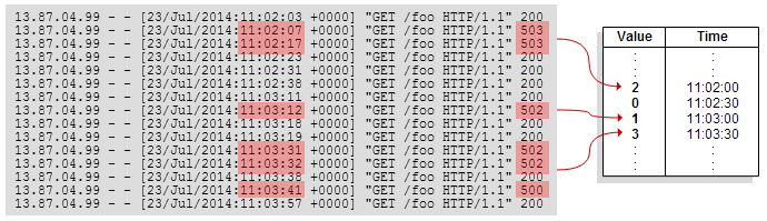
We can make this easy by precomputing the function for each point in time. In practice, we use 30-second resolution. Our data structure is simply an array of numbers per query, giving the numeric output of that query per 30-second interval. We call this array a timeseries. For example, suppose a user has a dashboard graph showing the rate of 5xx errors generated by a pool of web servers. We’ll create a timeseries which counts the number of errors in each 30-second interval:
Now, we can quickly generate a graph for any time period. (To graph long time periods, we also store a few redundant arrays using progressively coarser time intervals.) Using this data structure, the impossibly difficult problem of scanning terabytes of data in less than a second becomes rather simple.
Of course, we’ve traded one problem for another — the problem of building and maintaining timeseries. But unlike the original problem, this one is tractable.
Maintaining timeseries
To populate a new timeseries, we execute the underlying query across the entire retention period of the aggregated log. This is somewhat expensive, but we can do it in the background, and new dashboard or alert queries are infrequent.
To keep things up-to-date, we incrementally update each timeseries whenever a relevant log message arrives. For instance, if a new web access message has a status code in the range 500-599, we increment the counter in the “5xx errors” timeseries that corresponds to the appropriate time interval.
This introduces a new challenge: for each new message, we need to determine which timeseries it matches. Testing every message against every timeseries would require many millions of tests per second. We address this by taking advantage of the aggregate properties of dashboard and alert queries. These queries often use the same fields for filtering, such as hostname, metric name, or server tier. We can build a decision tree using these fields, and use it to quickly identify a short list of candidate timeseries which might match each log message.
A decision tree is organized around a root field―whichever field of the log message is most useful in narrowing down timeseries. Often, the root field will be the hostname. Timeseries which match messages from a specific host are grouped together; timeseries which aggregate across hosts go in their own group, the [any] group. Within each group, a new field is chosen, and timeseries are organized by that field. The subdivision continues until each group contains only a few timeseries.
To process a new message, we retrieve its value for the root field, and move to the subtree for that value. Eventually we arrive at a short list of timeseries, and evaluate the filter criteria for each timeseries to see whether it matches the event. At each level of the decision tree, we descend into two subtrees: the subtree corresponding to the message’s value for the decision field, and the [any] subtree.
Example
Imagine we have a dozen timeseries, which select messages according to the following (simplified) criteria:
host="frontend1" && metric="memfree"
host="frontend1" && metric="diskfree"
host="frontend2" && metric="memfree"
host="frontend2" && metric=diskfree"
host="backend1" && metric=memfree"
host="backend1" && metric=diskfree"
host="backend2" && metric="memfree"
host="backend2" && metric="diskfree"
pool="webapp" && status >= 400 && status <= 499
pool="webapp" && status >= 500 && status <= 599
pool="api" && status >= 400 && status <= 499
pool="api" && status >= 500 && status <= 599
We can organize these timeseries into a decision tree as follows:
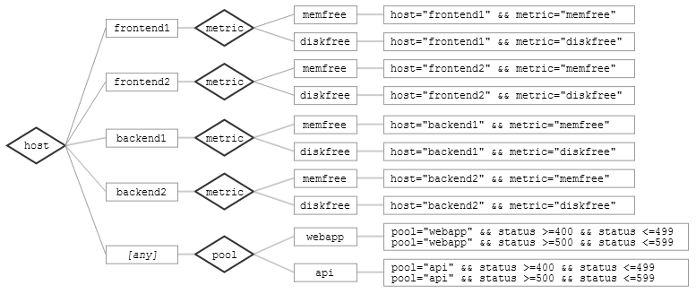
Now suppose we receive a log message with the following fields:
host=frontend1
metric=memfree
value=194207
From the root of the decision tree, we enter the host=”frontend1” and host=[any] nodes. From host=”frontend1”, we descend to metric=”memfree”, and match against the timeseries listed there. From host=[any], we find no applicable branches, and halt. We only have to test one of the 12 timeseries. In the worst case, for an event like {host=frontend1, metric=memfree, pool=webapp}, we’d test 3 timeseries.
Generating decision trees
Whenever you add an alert or edit a dashboard, Scalyr generates a new decision tree, optimized for the new set of timeseries. The decision tree is built using a simple greedy algorithm:
- Find all field names which are used in a == test in at least one timeseries. (In the example above, these are host, metric, and pool.)
- For each field name, partition the timeseries according to the value they require for that field. If a timeseries doesn’t require a specific value for the field, place it in an [any] group. Count the number of timeseries in each group, and find the largest group. In the example, the “host” field yields 4 groups of size 2, plus a group of size 4 (the [any] group). So the largest group has size 4.
- Build a tree whose root field minimizes the size of the largest group. In our example, both the host and metric fields have a largest-group-size of 4, so we could use either one. The pool field would have an [any] group of size 8, so we can’t use pool as our root field.
- Recurse on each subtree generated in step 3.
This algorithm performs quite well for us in practice. As an example, our internal production account has 1,996 timeseries. This generates a tree of depth 7, and the largest leaf node contains 15 timeseries. In the worst case, a log message might pass through 9 tree nodes, and be tested against 59 timeseries. (Remember that event processing can recurse down multiple tree branches―one field=value branch and one field=[any] branch at each level.)
This is a 33x speedup (from 1,996 timeseries to 59). In practice, the improvement is even greater, because 59 is the worst-case path through the decision tree. Most messages are compared against fewer timeseries.
Practical details
For completeness, a few loose ends I’d like to tie up:
- For each 30-second interval in a timeseries, we don’t actually store a single number. Instead, we store a compact histogram, summarizing the relevant numeric field of all log messages which fall in that time interval.
This is important for complex aggregations such as “99th percentile latency.” Suppose we’ve received 300 messages for a particular time interval, and the 99th percentile latency was 682.1 milliseconds. Then we receive a new message, with latency 293.5 milliseconds. How would we combine 682.1 and 293.5 to compute a new 99th percentile? We couldn’t; there isn’t enough information. We need a data representation that can be updated incrementally. For percentiles, a histogram fills the bill.
When generating a dashboard graph, we process each histogram to get the desired percentile. This is cheap enough to do on the fly.
- Updating all these histograms on a continuous, incremental basis generates a lot of data structure changes. It would be too expensive to persist each change to disk. Instead, we keep track of which histograms have changed, and flush them to disk every few minutes. On a server restart, we replay the last few minutes of logs to reconstruct the lost histogram updates. This adds complexity, but it’s worth it to keep per-log-message costs down. (Referring back to our design principle: new log messages are frequent, server restarts are rare.)
- When a new timeseries is created, we query the entire log database to populate it in the background, This is an expensive operation, which takes time to complete. If a user request arrives, we briefly leave off background processing to devote the entire server to the user request. We also populate the timeseries backwards (starting with the most recent data), to make it immediately useful for displaying dashboards.
The takeaway
Good algorithms can be helpful in improving performance, but it’s even more important to frame the problem correctly. Careful system design gave us search speeds of tens of gigabytes per second. Redefining the problem took us to terabytes per second. This involved rethinking the critical operation (retrieving numeric results for a predefined query), and pushing complexity to a less common operation (defining new alerts or dashboard graphs).
This is part of a series of posts on systems engineering and performance at Scalyr. For a look at frontend performance, see Optimizing AngularJS: 1200ms to 35ms. To read how we perform ad-hoc searches, read Searching 20 GB/sec: Systems Engineering Before Algorithms.
Using these techniques, we’ve been able to implement blazing-fast, reliable, flexible search of aggregated logs. We hope you’ll find these ideas useful in your own projects. If you’d like to see Scalyr’s performance in action, try it free or learn more about our hosted log monitoring service.